The Reserve Bank has begun using a new full-system macroeconomic model called MARTIN in policy analysis and forecasting. It is designed to be used as part of the Bank’s existing processes for forecasting and analysis, which use a range of information, models and staff assessments. MARTIN is already being used in these processes to help understand economic developments and quantify risks, and in time it will be used to extend forecasts beyond the usual two-to-three-year horizon.
Introduction
Since early 2016, staff at the Bank have been developing a new macroeconomic model for use in policy analysis and forecasting. The project was motivated by an external review of Economic Group’s forecasts and analysis (Pagan and Wilcox 2016). Kent (2016) outlined the key recommendations of the review, one of which was to develop and maintain a new macroeconomic model.
This article explains the rationale and goals of the newly developed model, known as MARTIN, as well as providing a broad overview of the model and its uses. MARTIN – which stands for MAcroeconomic Relationships for Targeting INflation – consists of a series of estimated equations that closely match the forecasting approach used at the Bank.[1]
Economic Modelling at the RBA
Models are simplified representations of reality that provide a framework for thinking about economic developments. They are useful because they help policymakers to:
discipline and organise their thinking
understand risks and assumptions, and communicate them clearly
produce forecasts and scenarios.
Because economic models are designed to simplify and help us understand the real world, they leave out potentially important variables and mechanisms. When building and using an economic model, a modeller needs to be clear about the relationships and causal mechanisms that matter to the policymakers they are designed to assist. The mechanisms that matter most for a central bank model are those that affect monetary policy through the economic cycle and over the longer term.
The Bank treats its models as one component of a wider toolkit for analysing economic developments and making policy decisions. The Bank maintains a range of single-equation and full-system models for forecasting and analysis (see ‘Box A: The Bank’s Suite of Models’ for more detail). Single-equation models look at a particular variable of interest while taking all other variables as given. For example, in the wage model in Bishop and Cassidy (2017) wage growth depends on the unemployment rate, the non-accelerating inflation rate of unemployment or NAIRU, inflation expectations and output prices.[2] Wage growth is the variable of interest, while all the other ‘explanatory’ variables are unexplained by the model. Single-equation models are much simpler to develop and to use than full-system models.
Full-system economic models look at many economic variables at the same time. This means fewer variables are taken as given. Instead, a wider range of variables are modelled explicitly, and the model is made up of a system of equations that are solved at the same time. Full-system models include relationships between explanatory variables, such as that between the unemployment rate and output prices in the wage example above. Full-system models also include feedback between economic variables. For example, lower wages may encourage businesses to hire more workers, which will then lower the unemployment rate and feed back to wages. Single-equation models miss these types of relationships and feedback mechanisms.
MARTIN is a full-system econometric model. The Bank also maintains a number of other full-system models. These include the multi-sector dynamic stochastic general equilibrium (DSGE) model documented in Rees, Smith and Hall (2016) and the suite of vector autoregression (VAR) models described in Gerard and Nimark (2008). The DSGE model is used primarily for scenario analysis, which is a useful input for economic forecasting and policy analysis. Likewise, the VAR models are used to produce forecasts each quarter as an input into the forecasting process. Often these models use different causal relationships to those that forecasters think about when formulating their forecasts, so they provide a useful point of comparison for the staff forecasts. The forecasting process is discussed further below.
Different types of models have strengths and weaknesses, and some are better suited to particular tasks. Single-equation models are simple and flexible, but they are limited in scope and lack feedback mechanisms. DSGE models are built on a consistent theoretical framework of optimising households and firms, which provides a clear interpretation of the causal mechanisms within the model and an explicit role for forward-looking expectations. A weakness of DSGE models is that they often do not fit the data as well as other models, and the causal mechanisms do not always correspond to how economists and policymakers think the economy really works. In order to more easily manage these models, they typically focus on only a few key variables, which can limit the range of situations where they are useful.
The key strength of full-system econometric models like MARTIN is that they are flexible enough to incorporate the causal mechanisms that policymakers believe are important and fit the observable relationships in the data reasonably well. They can also be applied very broadly to model a wide range of variables. This flexibility reflects that the model is not derived from a single theoretical framework, which can make causal mechanisms less clear than in DSGE models. The model might capture an empirical relationship that exists in the data, but the cause of this might not be well understood. This means that developments may be more difficult to interpret and assumptions may need to be made about the mechanisms that are at work. If the true causal mechanisms are not correctly captured, empirical relationships may be unreliable over time or developments may be interpreted incorrectly. See Wren-Lewis (2018) for a discussion of different modelling approaches and the advantages of full-system econometric models like MARTIN.
Box A: The Bank’s Suite of Models
The Bank employs a suite of economic models. Figure 1 visualises the models used in the Bank and locates MARTIN in a modelling taxonomy. Models can be classified along two axes. One axis describes how much the model structure is driven by economic theory as opposed to empirical relationships observed in the data. Theory-driven models require choices among competing theoretical frameworks. These choices affect the behaviour and predictions of a model, which should be taken into account when applying them to real-world situations. The other axis describes the scope of the model, from the narrow focus of a single-equation model to the broad scope of a full-system model of the whole economy. MARTIN is broad in scope. It incorporates economic theory by using economic intuition to guide its longer-run properties, but it is also designed to capture relationships visible in the data, particularly in its short-run dynamics.
VAR, SVAR and FAVAR: Gerard H and K Nimark (2008), ‘Combining Multivariate Density Forecasts Using Predictive Criteria’, RBA Research Discussion Paper No 2008-02.
DSGE: Rees D, P Smith and J Hall (2016), ‘A Multi-sector Model of the Australian Economy’, Economic Record, 92(298), pp 374–408.
AUD ECM: Hambur J, L Cockerell, C Potter, P Smith and M Wright (2015), ‘Modelling the Australian Dollar’, RBA Research Discussion Paper No 2015-12.
Phillips Curve: Cusbert T (2017), ‘Estimating the NAIRU and the Unemployment Gap’, RBA Bulletin, June, pp 13–22.
Mark-up model: Norman D and A Richards (2010), ‘Modelling Inflation in Australia’, RBA Research Discussion Paper No 2010-03.
Asset pricing model: Fox R and P Tulip (2014), ‘Is Housing Overvalued?’, RBA Research Discussion Paper No 2014-06.
Exports ECM: Cole D and S Nightingale (2016), ‘Sensitivity of Australian Trade to the Exchange Rate’, RBA Bulletin September, pp 13–20.
Okun’s Law: Lancaster D and P Tulip ‘Okun’s Law and Potential Output’, RBA Research Discussion Paper No 2015–4
MARTIN’s Development and Use
The goal for MARTIN is different to the goals of the Bank’s other full-system models. MARTIN is designed to systematise the existing methods and equations used in the Bank for forecasting and analysing the economy. MARTIN’s role is to bring together the analytical frameworks of the Bank’s analysts, rather than a framework that acts as an independent check. This meant developing a model that corresponds closely with the way analysts and policymakers at the Bank think about the economy. This objective drove the modelling approach and scope, as well as the choice of variables and causal mechanisms in the model.
Why this type of full-system model?
Many central banks use full-system models. The design of these models reflects the purpose of the particular model and the priorities of each central bank.
MARTIN’s goal is to enhance the Bank’s current framework by
extending forecasts beyond the usual two-to-three-year forecast horizon
producing scenarios and other analysis to quantify risks
improving our understanding of how the forecasts fit together.
DSGE models are currently the most widely used class of full-system models at central banks.[3] But a DSGE model was not the appropriate choice for MARTIN because the economic mechanisms in such models do not align well with the current analytical framework used for forecasting and analysis.
Instead, we have built MARTIN as a full-system econometric model. This approach is similar to a number of contemporary models used by other central banks, including FRB/US, used by the Federal Reserve (Brayton, Laubach and Reifschneider 2014), and LENS, used by the Bank of Canada (Gervais and Gosselin 2014). It is also similar to some previous models of the Australian economy, including AUS-M (Downes, Hanslow and Tulip 2014) and its predecessor, TRYM, which was developed by the Australian Treasury (Commonwealth Treasury 1996).
A model that is consistent with the Bank’s analytical approach
Analysts at the Bank monitor and seek to understand economic developments as they unfold. One aspect of this broader analysis is producing quarterly forecasts that feed into the forecasts published in the Statement on Monetary Policy. The published forecasts summarise an extensive process in which analysts incorporate incoming data and other information, such as reports from the Bank’s liaison program, assess the relevance of new events, construct forecasts for a large number of economic variables, analyse various scenarios and consider a range of risks to the outlook. The forecasting process was described in more detail in Kent (2016).
To assist in their forecasting and wider analysis, analysts will typically use a range of single-equation models that embody the key relationships for the variables they monitor. For example, a housing analyst uses equations where dwelling investment depends on interest rates and recent housing price growth.
To make MARTIN as consistent as possible with the Bank’s current approach to forecasting and analysis, we mirrored the staff’s single-equation models where we could. For example, MARTIN’s dwelling investment equation includes variables that influence staff forecasts like interest rates and housing price growth. MARTIN’s equation also includes a long-run relationship where dwelling investment maintains a stable share of GDP over time, which is both evident in the data and consistent with many theoretical models. The long-run properties of the equations are more important for MARTIN than the usual forecasting equations that have at most a 12-quarter forecast horizon.
Equations are not the best tool for forecasting all economic variables. For example, business investment is particularly hard to model using economic drivers. Nonetheless, a full-system model needs an equation for each variable, so we developed an equation for business investment based roughly on Cockerell and Pennings (2007). In practice, forecasters consider model output alongside a large range of other information, for example, business surveys and liaison information. When additional information like this is available, it can be incorporated into MARTIN by adding judgement to the equation (that is, imposing equation residuals).
For MARTIN to be integrated with the Bank’s policy process it needs to be well understood by staff and policymakers. This can be a problem for very complicated models that are only understood by a small group of specialists. To ensure MARTIN would be well understood, we kept it as simple as possible and designed and developed it in close consultation with the forecasting staff who will be the main consumers of this model’s output.
MARTIN at a Glance
MARTIN is a full-system econometric model built using an error-correction framework. The model’s equations are estimated independently of each other (in the same way as the single-equation models used by staff in forecasting) and are then combined to form a model system. When the model is run, the equations in the system are solved simultaneously. This means that model simulations capture the interdependencies and feedback mechanisms in the model equations.
Equation design
Most key behavioural equations in MARTIN are modelled using error-correction models. An equation is considered ‘behavioural’ if it captures important aspects of economic behaviour (for example, how much households spend or how prices are set).
Error-correction equations are used because they can match empirical regularities in the data, while having stable long-run properties. Under this approach, economic variables are assumed to revert (or ‘error-correct’) to long-run growth paths based on cointegrating relationships in the data that are consistent with economic intuition.
A group of cointegrated variables tend to move together over time. They might deviate temporarily, but over the long run they follow a reliable relationship, so any deviation will eventually dissipate as this relationship is restored. Error-correction equations use the predictive power of these reliable relationships. In some cases, long-run relationships are assumed to vary over time, allowing the model to capture changes in these relationships, perhaps as a result of structural change in the economy.[4]
The long-run relationships in an error-correction model ensure that the whole model system stabilises in a plausible way. The specification of the long-run relationships combine empirical relationships in the data with economic intuition, which is used to guide what economic relationships might be considered ‘plausible’. This helps to ensure that results are sensible and interpretable. For example, in MARTIN, the level of the household saving rate can move around based on relationships in the model, but we restrict the long-run behaviour of consumption to ensure that growth in household spending cannot permanently exceed income growth.
In the short term, economic developments can drive variables away from their long-run relationships. The effects of these short-term drivers are estimated to match the persistence and empirical relationships observed in the data, provided those relationships are plausible based on economic intuition.
The model captures a range of endogenous and exogenous variables. Variables that are affected by other model variables are called ‘endogenous’. Inflation is considered an endogenous variable because it responds to the unemployment rate and import prices, which are also modelled. ‘Exogenous’ variables are those that affect other variables in the model but are not themselves affected by other variables. The path for global growth is considered exogenous because it is not affected by any other model variables.
In addition to behavioural equations, a number of endogenous variables are constructed based on accounting identities (for example, GDP is the sum of its expenditure components). While exogenous variables are not themselves affected by other model variables, they still need to be modelled. Sometimes paths for these variables are imposed using information from outside the model; sometimes they are modelled using simple equations.
Scope of the model
MARTIN has been designed to provide a framework to interpret economic developments and assist policymakers. This objective affected the scope of the model. In particular, variables that feature in the transmission channels of monetary policy are modelled comprehensively, including interest rates, the exchange rate, components of real GDP, the labour market and inflation.
In a recent RBA Bulletin article, Atkin and La Cava (2017) outlined some of the transmission channels of monetary policy and explained how they work. MARTIN incorporates similar mechanisms to those described in that article and can provide quantitative estimates that incorporate feedback mechanisms in the economy. The channels of monetary policy can be considered together – an important feature for actual policy analysis.
To keep the model relatively simple, some aspects of the economy – for example, fiscal policy and the financial sector – are modelled in a more rudimentary way, at least in this first version of the model. Nonetheless, MARTIN is still quite large, comprising 33 behavioural equations.
Some parts of the economy are modelled in a more disaggregated fashion than others, to incorporate key features of the Australian economy. For example, business investment is split into mining and non-mining, reflecting the importance of the resources sector (which has evolved differently from the rest of the economy over the past decade or so). For the same reason, exports are modelled in a relatively disaggregated way. On the other hand, foreign variables are aggregated, reflecting the domestic focus of the model. Only a few key foreign variables are included, capturing world influences on the domestic economy. Including more disaggregated foreign variables would add complexity without much benefit.
Many variables are assumed to be exogenous, not because they are unimportant, but because it is reasonable to assume that they are unaffected by the rest of the model, or because modelling them endogenously would add complexity that is not needed. We model foreign variables exogenously because the Australian economy does not have a large influence on the world economy. Some variables are modelled in a relatively simple way because modelling them in a more detailed way again adds complexity without much benefit. This is the case for very unpredictable variables, such as commodity prices. Some domestic variables are also modelled exogenously, including population and productivity growth, the neutral interest rate and the NAIRU. These variables reflect uncertain, slow-moving trends that are difficult (or quite complicated) to model using other variables in the model.
An overview of MARTIN
To capture key elements of monetary policy transmission and features of the Australian economy, MARTIN includes detailed modelling of GDP expenditure components, the labour market and determinants of inflation (Figure 2). GDP depends on decisions by domestic firms and households and international trade. Households’ decisions are affected by their income and balance sheet position. Economic activity affects demand for labour and the degree of spare capacity (or slack) in the labour market.
Wages and prices provide a link between the labour market and the nominal side of the economy. Spare capacity in the labour market, output prices, and inflation expectations determine the rate of wage growth. Wages and import prices (which are affected by the exchange rate) affect input costs of firms. Input costs and capacity pressures flow through into output prices and the trimmed mean consumer price index (CPI).
The cash rate is set using a monetary policy rule. The baseline rule is a backward-looking Taylor rule: policy responds to deviations of year-ended trimmed mean inflation from target and the unemployment gap. In reality, monetary policy is forward looking. In MARTIN, monetary policy is forward looking to the extent that recent values of inflation and the unemployment rate are informative about the future. For some model simulations, the cash rate may be varied from what the rule suggests. But for the model to converge to a stable steady state, the cash rate must eventually respond endogenously to bring inflation back to the midpoint of the target band and the unemployment rate to the NAIRU.
In MARTIN, the cash rate affects the economy in three key ways:
Exchange rate: When the cash rate falls, the exchange rate depreciates. The depreciation boosts export competitiveness, which increases exports. Likewise, exchange rate depreciation raises import prices, which reduces import volumes. Higher import prices increase inflation through the imported content of the CPI.
Asset prices: A lower cash rate boosts housing prices and equity prices. Lower mortgage rates encourage households to purchase new and established housing, and mean that households can service more debt. This increases the value of housing and household borrowing. Lower interest rates and higher housing prices make dwelling investment more profitable, while increases in housing wealth boost consumption.
Households and businesses: When the cash rate is lowered, this reduces interest payments (and receipts), boosting household income and consumption overall because households collectively hold more interest-bearing debt than assets. Reductions in the cash rate also boost short-term consumption directly and increase non-mining business investment via lower costs of funding, but these effects are estimated to be small.
These channels together mean that a decrease in the cash rate provides a short-term boost to GDP growth due to higher net exports, dwelling investment, consumption and business investment. Stronger GDP growth boosts income, further increasing business investment and consumption.
Stronger GDP growth increases labour demand and lowers the unemployment rate. Reduced unemployment lowers the amount of spare capacity in the labour market and puts upward pressure on wage growth. Higher wages, increased import prices (due to exchange rate depreciation) and capacity pressures put upward pressure on prices in the economy. As a result, trimmed mean CPI inflation increases.
Increases in wage growth and inflation are persistent, which may reflect the role of backward-looking expectations in wage- and price-setting behaviour. Forward-looking expectations are included in the inflation and wage equations, but they are not modelled endogenously. This means that monetary policy has no effect on expectations for wages and prices in the model. However, expectations can be an important channel for the transmission of monetary policy – for example, firms might change their prices in response to a decrease in the cash rate in anticipation of higher future inflation. Improving our modelling of expectations and developing a forward-looking policy rule are key areas for further work.
How MARTIN is Used
MARTIN has been designed to assist in forecasting and policymaking at the RBA in a number of practical ways.
MARTIN can be used for scenario analysis to consider the implications of risks that are relevant for policy. Scenario analysis involves running the model using alternative paths for one or more of the variables, then comparing the implied outcomes with a baseline forecast. By looking at the differences between alternative scenarios and the baseline, MARTIN can illustrate the economy-wide effects and policy implications of different scenarios. For example, we might consider the effects on unemployment, inflation and the cash rate from alternative paths for commodity prices.
Scenario analysis is an important input into the forecasting process and it can be used for other policy analysis. The model can be used to understand and quantify answers to policy-relevant questions. For example, MARTIN could be used for counterfactual analysis to understand the economy-wide effects of the resource investment boom as in Downes, Hanslow and Tulip (2014). The model could also be used for policy analysis, including ‘optimal control’ exercises, in which optimal policy paths are estimated using the model, based on different assumptions for policymakers’ preferences.
MARTIN can be used to produce its own model-based forecasts, with and without imposing assumptions and additional judgement. This means we can use the model to extend the staff forecasts over a longer time horizon, so that we can analyse long-term implications of the staff forecasts. A model is particularly useful for understanding developments over longer time horizons because feedback mechanisms in the economy become more important and fewer leading indicators are available. The economic intuition built into the long-run relationships in MARTIN means it can be used for these forecast extensions.
We can also use MARTIN to understand the staff forecasts. In particular, we can match the forecasts that are produced by staff at the RBA using single-equation models, other indicators and a range of non-model information, such as insights from liaison, by adding judgement (with equation residuals). These equation residuals can reflect anything that is not explained by the model and they may be difficult to interpret. Understanding how forecasts deviate from the model is useful for critically evaluating them. Deviations are not necessarily wrong because models are simplifications of reality, but quantifying large deviations is a useful discipline and may flag areas that would benefit from further analysis.
Once the staff forecasts are matched, we can use MARTIN to decompose and understand the outlook based on the relationships captured in the model. For example, we can understand the direct drivers of inflation, such as input costs, and decompose these into their ultimate drivers, like changes in world commodity prices or consumption behaviour. MARTIN can also be used to produce confidence intervals around the forecasts, based on uncertainty implied by the model residuals.
MARTIN’s Future
The Bank has been using MARTIN for scenario analysis and analytical work since the middle of 2017. In time, MARTIN will be used internally to extend forecasts to understand and analyse the outlook beyond the two-to-three-year published forecast horizon.
But while the Bank is benefiting from having a new full-system model, not all of the model’s details are bedded down. Indeed, building the new model is simply the start of an ongoing process. There is still much to do to understand and implement MARTIN and develop the model further; reviewing the model’s features in light of new information will be a continuous process.
We are continuing to investigate the model’s properties and intend to integrate the model further with our forecasting and policy processes. For example, we plan to use the model to analyse staff forecasts and to consider the effects of structural change over the long term. We will also continue to develop and refine the model. There are a number of ways that we can extend the model to add richness to its analysis. For example, in future work, we may add a more developed supply side to the model or incorporate expectations formation.
We will continue to publish updates and details on the model, including a detailed description of the first version of MARTIN, over time.
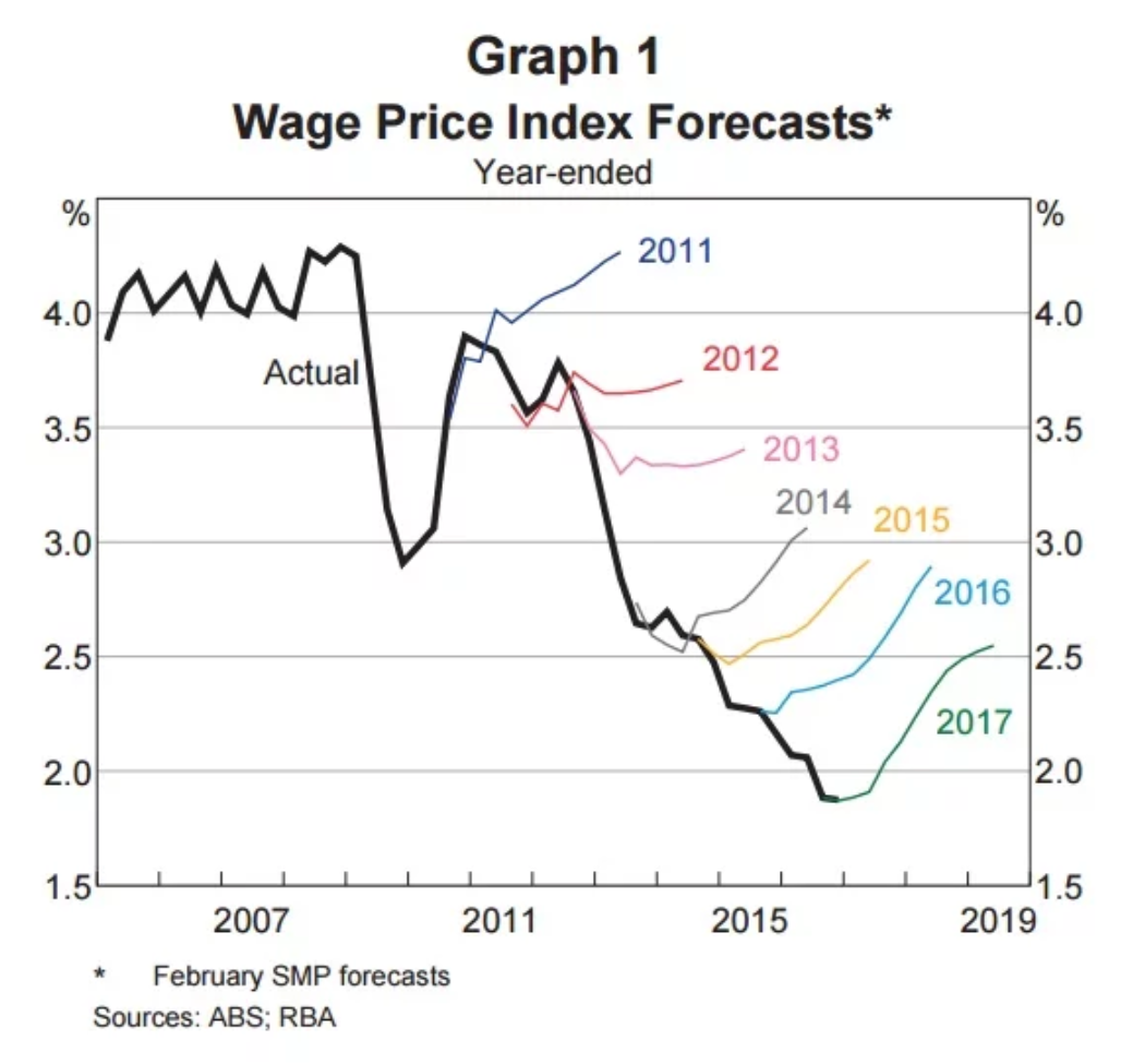
Built by the RBA it almost certainly has growth perpetually moving up to trend, inflation returning to target, wages up and unemployment down:
David Llewellyn-Smith is Chief Strategist at the MB Fund and MB Super. David is the founding publisher and editor of MacroBusiness and was the founding publisher and global economy editor of The Diplomat, the Asia Pacific's leading geo-politics and economics portal.
He is also a former gold trader and economic commentator at The Sydney Morning Herald, The Age, the ABC and Business Spectator. He is the co-author of The Great Crash of 2008 with Ross Garnaut and was the editor of the second Garnaut Climate Change Review.