As H&H has pointed out, Former Treasurer Peter Costello, made some good points today about the challenges ahead for the economy and property but he also backed-up Joe Hockey’s poor effort yesterday, claiming that there is no housing bubble because there is a shortage of supply. From The AFR:
“For a western developed country, Australia’s population growth is very strong,” Mr Costello said.
“So we have to factor that housing supply is not meeting demand. It’s important the public understands this”…
“If you speak to anyone outside Australia as I do, they will ask if the Australian residential property market is overvalued… It is the first thing any economic investor will ask”.
“They say that using multiples against world standards… But we are growing so fast, faster than the Mexicans, Argentinians, South Africans”…
“Building a house is comparatively cheap… What is expensive in Australia is land. We have increasing demand but quite a restrictive supply of land and as a result, prices are high”.
“Houses are so expensive because the government has the control on land…”
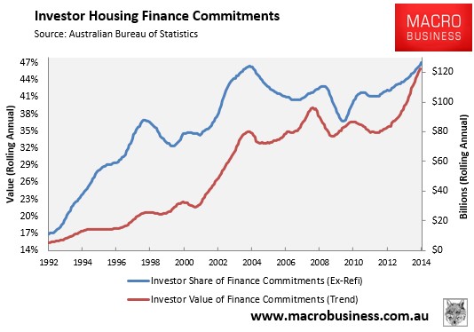
While I obviously agree with Costello on Australia’s ridiculous land prices, brought about in-part due to government land-use policy, I’m not sure how Costello can ignore the record high level of investor speculation, most of which is negatively geared:
Moreover, how do Costello and Hockey explain why markets with similarly restrictive land-use policies to Australia – Ireland, Spain, California, Florida, Arizona, and Nevada – experienced large booms and then busts? How is this possible in their world?
Both Joe Hockey and Peter Costello need an economics lesson. As I have explained previously, unresponsive housing supply results in greater house price volatility – both on the way up and the way down. Such a situation can be explained using basic supply and demand analysis, as shown in Figure 1:
Q0 and P0 represent the initial equilibrium situation in the housing market. Initial demand is provided by D0, whereas supply is shown as either SR (restricted) or SU (unrestricted), depending on whether land supply constraints exist.
Following an increase in demand, such as a surge of investors following changes to tax rules (e.g. Australia’s CGT reduction in 1999), the demand curve shifts outwards from D0 to D1. When land supply is restricted, house prices rise sharply from P0 to PR. By contrast, when supply is unrestricted, prices rise more gradually from P0 to PU.
The situation works the same way in reverse. For example, if there was a sharp fall in demand, say following a contraction in credit availability or a sharp decrease in Australia’s Terms of Trade, causing demand to fall from D1 to D0, then prices tend to fall much further when land supply is constrained.
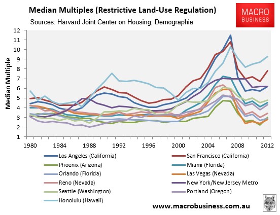
This was illustrated perfectly in the US bubble. There, markets that operated restrictive land use policies and regulations that hindered market from supplying affordable homes in a timely manner experienced large booms and busts, a sample of which are shown below:
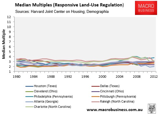
By contrast, those markets that operated liberal land-use policies – and in turn kept land prices low and allowed the market to supply homes relatively quickly and affordably – experienced much lower price volatility (see next chart).
The key point of this analysis is to show that declines in demand can bring sharply falling house prices even when supply is constrained and housing shortages exist and restrictive supply combined with easy credit are key ingredients of housing bubbles.