
The sale price of homes is not the economic price of housing. Prices, in the economic sense, are the relative cost of consuming newly-produced goods and services.
The economic price of housing is therefore the rental price. It represents the price of being housed today. The rental price is what goes into consumption price indexes. It goes into the national accounts to represent housing service production. It is what standard economic theory says is the price of housing.
The sale price of a house represents the purchase of a perpetual stream of housing services. In essence, you are buying the right not to have to rent a home from someone else.
Why is it important that the sale price of a house is not its economic price?
Because sale prices of housing can rise while their economic price falls. The economic price of housing translates into a sale price via other factors.
So how is the sale price of housing determined?
The asset pricing model
Converting the value of a flow of uncertain future income flows into a capital value today is an imperfect procedure, relying on estimates of risk, uncertainty and growth prospects. But we can for now ignore these judgements to demonstrate how the ingredients that create an asset price from the value of an income stream fit together.
Housing asset prices can be reflected by the following formula.
Asset price = (gross rent – ongoing costs) / (risk-adjusted return + property tax rate – growth expectations)
There are hence five ingredients in asset prices, of which only one is the economic price in the form of the annual rent. This is why housing asset prices can diverge so significantly from rental prices.
Let us go through each ingredient.
- Gross rent is the total amount a renter would have to pay to occupy the home for a period. It is the economic price of housing.
- Ongoing costs include upkeep of the house—the maintenance required to sustain its current quality over time (depreciation)—as well as other ownership costs such as taxes and fees that are not levied as a fixed rate on the property value.
- The risk-adjusted return is the rate of return buyers are will to pay for that property based on their assessment of market alternative investment returns, and the relative rate of risk of buying this house. For example, if you can get a 5% return on you money in the bank from interest, and buying this house is seen as much risker than bank deposits, then this return will be something above 5%, say 8%.
- The property tax rate is the rate per dollar on the total property value that is required to be paid in taxes. In most US cities and states, property taxes are levied on the full asset value of the house and land, whereas in other places like Australia, these taxes are levied only on the land value component. I have adopted the US approach here for simplicity.
- Growth expectations reflect the rate at which much buyers expect rents or prices to rise in the near future. For example, you may buy a house to avoid paying $20,000 per year rent, but rents might be rising at 5% per year. Next year, your current house purchase saves you $21,000, and it saves you $22,000 the following year.
- We are going to simplify this model for now by pretending that growth expectations are zero. This avoids the part of the recipe that leads to big swings in the value of housing that usually self-correct over time. We will also pretend that the risk-adjusted return is best captured by the prevailing mortgage interest rate. Once you see the logic if the model, you can easily tweak these assumptions yourself to see their effect on asset prices.
The cost of buying vs the cost of renting
Here is an example of the asset pricing model in action. A house has the following characteristics.
Rent is $20,000 per year
Ongoing costs are $5,000 per year
Mortgage rates (risk-adjusted return) are 6%
The property tax rate is 0.5%
Growth expectations are zero.
The sale price of this home will be roughly $231,000 according to the asset pricing formula [(20,000-5,000)/(0.06+0.005) = $231,000].
What this means is that you will be equally well off economically—i.e. you will spend the same each year—if you borrow the full house price amount and buy it as you would be renting it. We can add up the annual costs of buying to seeing that it is the same as renting.
Interest = $13,850 ($231,000 x 0.06)
Ongoing costs = $5,000
Taxes = $1,150 ($231,000 x 0.005)
Total = $20,000
You might notice that I have only considered the interest cost of a mortgage, not the total repayment. But paying the principle of the house is not an economic cost. It is an asset investment just like paying listed equities is an investment, not an economic cost.
Our homebuyer in this situation is paying a $20,000 economic cost of housing. But if they pay the principle of their loan over 30 years, the mortgage repayment is $16,780 per year, or $2,930 more than the interest alone. Their out-of-pocket expenses are $22,930, but that include the purchase of $2,930 of housing equity each year.
The effect of low interest rates
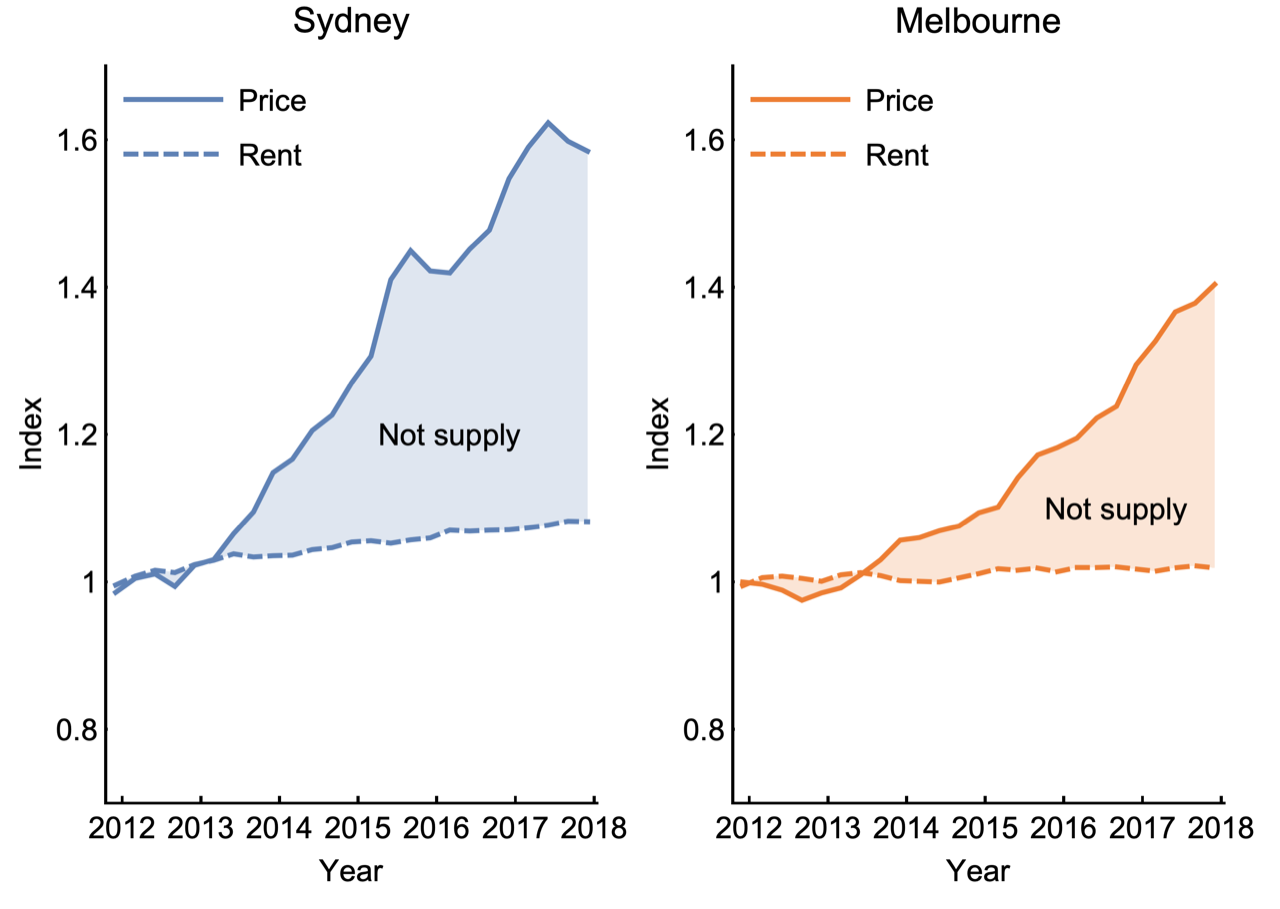 If recent sale price changes are not due to rents, then they must be due to one of the other ingredients in the asset pricing model.
 We can eliminate the ongoing costs of upkeep. Construction costs have been steady, and fixed fees and charges also have seen little variation. Property tax rates are also relatively unchanged, at least in Australia. Note also that higher property taxes reduce asset prices.
We are now down to two factors—the risk-adjusted return and growth expectations.
It could be that buyers of housing have increased their expectations of rental growth. Though after a decade of flat or falling rents, rental growth expectations should certainly have been curtailed, rather than increased.
This leaves only the interest rate. To me, this is the big story for housing prices over the past two decades globally.
We can take our previous example dwelling where we calculated its value to be $231,000 when mortgage interest rates were 6%. Now, mortgage interest rates are closer to 2%. At what price does buying cost the same as renting at this much lower rate?
Again assuming zero growth expectations, our asset pricing formula is (20,000 – 5,000) / (0.02 + 0.005) = $600,000. That’s a 160% increase in sale price, while the economic price of house remains unchanged.
We can check this calculation to ensure that the economic cost of buying at this price remains the same as before.
Interest = $12,000 ($600,000 x 0.02)
Ongoing costs = $5,000
Taxes = $3,000 ($600,000 x 0.005)
Total = $20,000
Notice that the interest paid on a mortgage is actually lower in this case, though the annual taxes are higher due to the higher sale price.
What about property taxes?
First, we can see the effect of property taxes in our high 6% interest rate scenario. Recall that the asset price with a 0.5% property tax rate was $231,000. If we now put a 2% property tax rate in our asset pricing equation, the house is worth $187,500. Compared to this high-tax region, the asset price of the same house in a low-tax region will be 23% higher. That is a huge difference. Yet the economic price of housing is the same.
In the low interest rate scenario our house was worth $600,000 in the 0.5% low property tax area. If we plug in a 2% property tax rate and a 2% interest rate we get a value of $375,000 in the high-tax region. The sale price is now 60% higher in the low tax area for the same economic price of housing. The low interest rate environment amplifies the price effect of different property tax rates.
We can see the components of the economic price in the high property tax area in the low interest rate scenario below.
Taxes = $7,500($375,000 x 0.02)
Total = $20,000
We can therefore use the asset pricing model to predict that the recently-announced reductions in property tax rates in Harris County (Houston) will fuel price growth in the current low interest rate environment. We can also predict that states like Texas, with comparably high property tax rates (often 2% and above) will have even greater housing asset price divergence compared to regions with low (sub 1%) property tax rates.
Predicting strange price differences
Strange house price differences make more sense through the lens of asset pricing.
Here is an example of the types of strange price differences commonly noted. Here are two houses where the asset price seems unrelated to the quality or size of the dwelling.
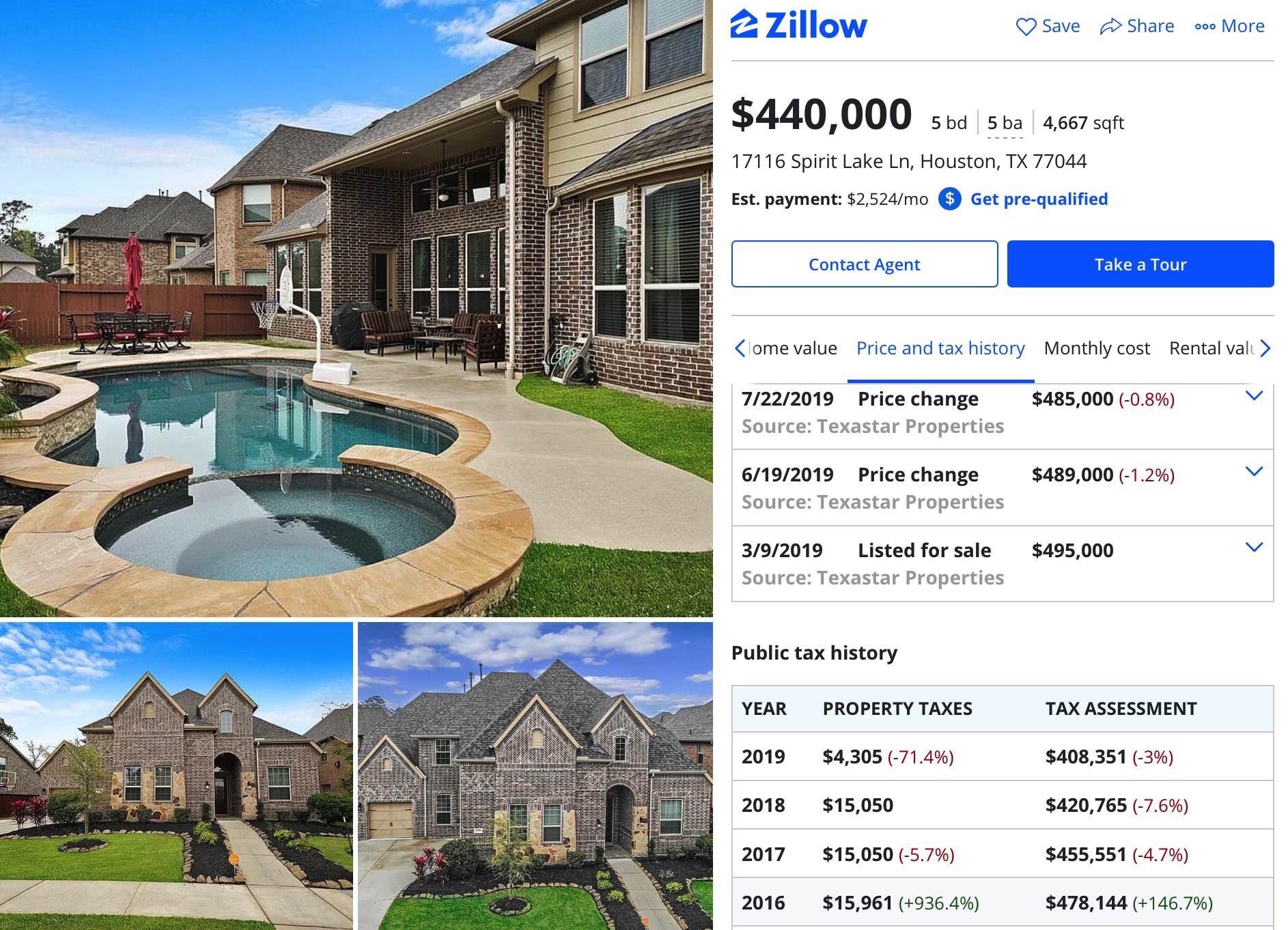
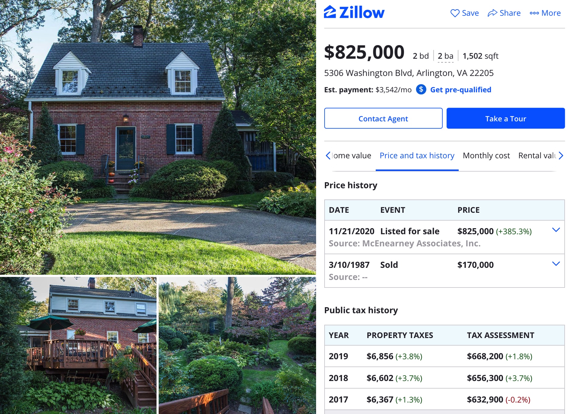
Can asset pricing make sense of the fact that the much smaller home is worth nearly double the much larger one?
It can.
We can even acknowledge that the economic price of the larger home is much higher, despite location difference. But this does not have to translate into a higher asset price.
The large home, House 1, might have the following characteristics.
Gross rental per year: $40,000
Property tax rate: 3%
Ongoing/upkeep per year: $10,000
The high upkeep costs (aka depreciation) come from its size and features, such as the pool. Notice that property taxes are around $15,000 per year for this dwelling, which is over 3%.
The smaller home might have the following characteristics.
Gross rental per year: $30,000
Property tax rate: 0.8%
Ongoing/upkeep per year: $5,000
Notice the much lower property taxes and upkeep costs. This has a big effect when converting the economic price into an asset price.
I’m going to apply a 2% mortgage interest rate to the asset pricing formula to show what price to expect for these two homes.
House 1
Price = $40,000 – $10,000 / (0.02 + 0.03) = $600,000
House 2
Price = $30,000 – $5,000 /(0.02 + 0.008) = $893,000
Although the economic price, the rent, is 33% higher for House 1, this doesn’t translate to asset prices. In fact, House 2 is worth nearly 50% more than House 1 under these conditions (my price estimate is a bit on the high side for both as I’m using a round 2% and ignoring any difference in other asset pricing factors).
House 1
Interest = $12,000 ($600,000 x 0.02)
Ongoing costs = $10,000
Taxes = $18,000($600,000 x 0.03)
Total = $40,000
House 2
Interest = $17,900 ($893,000 x 0.02)
Ongoing costs = $5,000
Taxes = $7,100($893,000 x 0.008)
Total = $30,000
If you are not looking at housing sale prices through an asset pricing lens, these strange house price differences will only seem to get worse as we enter a super-low interest rate period. Many people will mistakenly attribute the difference in asset price to physical and regulatory factors, like zoning. But if these factors do affect housing, the must do it through their effect on the economic price, the rent, not the asset price.