
This is the question I answer in a new working paper entitled A Housing Absorption Rate Equation. I sketched out some of my initial thinking on this topic in a blog post earlier this year. Here I want to explain this new approach more clearly and show why it is important for the housing debate.
Why is this important?
Economic analysis of housing supply is usually based on a one-shot static density model. In this model, landowners choose a housing density that maximises the value of their site. The density that achieves this is where the marginal development cost of extra density equals the marginal dwelling price. Every landowner does this instantly. There is no time in the model. It just happens.
But optimal density (dwellings per unit of land) is not optimal supply (new dwellings per period of time).
Despite this conceptual confusion, radical town planning policy changes have been proposed around the world. By allowing higher-density housing, proponents of these policies expect that the rate of new housing supply will increase enormously, reducing housing prices.
I wouldn’t be that confident. It is not clear that the economic factors that influence the optimal density are the same ones that affect the rate of new supply, or what is known as the absorption rate.
What factors influence the optimal rate of supply?
To answer this, we break apart the time dimension of the development problem. In a dynamic setting, the economic value from a sequence of dwelling lot sales is maximised when delaying the marginal sale into the next period makes you equally as well off as selling that dwelling today.
The economic factors that influence the absorption rate are those that change the relative gains from selling now rather than delaying and selling later. Let us think about the motivating puzzle of a housing developer selling new lots.
From the perspective of the second period, if you sell a lot today, you get the interest rate on the lot value, plus you avoid any taxes on that lot value.
If you sell on that later period, you got the value gain of the lot. This value gain comes from the market at large (i.e. the trade of existing dwellings) but is also affected by your own sales in the first period. Sell more now, get lower price growth and hence a lower price in the next period. The net price gain is, therefore, market demand growth minus your own-price effect on that price growth.
The optimal point is where you are equally well off making the same number of sales in the current period and the next period.
The result of the dynamic supply problem is this equation.
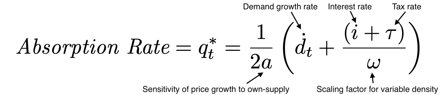
Let’s walk through this one parameter at a time.
Price growth sensitivity to own-supply, a
The first parameter of interest is the own-price effect, a. A higher a means that each sale today has a larger effect on price growth. It’s a measure of the “thinness” of the demand side of the market. Since a is the denominator, it means that the thinner the market, the lower the optimal rate of sales.
Market demand growth rate, d
When demand growth is high, you sell more. This makes sense. You sell into a boom and withhold sales during a bust. This is important because one argument for relaxing density restrictions is that new supply would occur at such a rapid rate that prices would fall. But falling prices reduce supply. There is hence a built-in ratchet effect in housing supply dynamics.
Interest and land tax rates, i and 𝜏
These two rates work in combination. The interest rate is the gain you get on the cash from selling a lot today, and the land tax rate is a cost you avoid from selling today. The gain from not owning land (i.e. selling it) is the interest rate and the land tax rate, which is positively related to the optimal absorption rate.
The efficiency of higher density, ω
The final piece of the puzzle is the ω parameter. This parameter captures the idea that if you delay selling a lot you can change the density of development in response to rising prices. Remember that static density model? This is where it is useful. It shows that if prices rise, undeveloped sites rise in value more than the dwelling price because the higher price justifies denser housing development.
I show this in the below diagram. At price Pt the optimal density is Dt, and the site value is the orange shaded area (the dwelling price minus the average development cost times the number of dwellings).
If prices rise to Pt+1, then the optimal density is now Dt+1. The value gain for the site is not just the area marked A, which it would be if density was fixed. It is the area A plus the area B, minus the area C. Since B > C this means the site value rises more than the dwelling price change. The ω term captures how much bigger A + B – C is than A. When ω is 1, it means that density is constrained to Dt and site value rises only by the dwelling price change. Flatter cost curves create a larger ω.
The important thing to remember is that constraining density makes ω smaller (holds it at 1). This increases the optimal absorption rate because it reduces the gain to delay that comes in the form of the ability to vary housing density.

Where does this model leave us?
Having a simple absorption rate model allows housing researchers to think more clearly about the economic incentives at play for housing suppliers. It allows us to break away from the “density = supply” confusion. Instead, it focusses attention on the key issue of the relative returns to delaying housing development.
Any policy that increases the cost to landowners from delaying housing development will increase the rate of new housing supply. For example, higher land taxes and interest rates.
Another way to increase the cost (reduce the benefit) of delay is restricting density. This goes against the intuition of most housing researchers, but the economic effect is real.
Think about it this way. You announce a policy that will limit density in an area to half of what is currently allowed in five years time. What happens? You get a housing development boom as projects are brought forward in time. You massively increased the cost of delay.
It is obvious that planning controls change the shape of cities. They reduce housing density in some areas and restrict certain uses in others. That’s what planning does. But how this translates into an effect on the rate of new housing supply across a city is far more difficult to ascertain. This model goes some way to helping housing researchers clarify their thinking about the economic incentives at play in housing supply, instead of relying on intuition and inappropriate static models.