

I was motivated by this article in The Economist about housing costs in London to really dig down to how most economists think about housing supply and land markets. Today I want to share a simple model I use to help understand compositional effects on measures of land and housing markets, and subsequently the reliability of particular measures for understanding potential supply issues.
The model
At time=0 a city has 20 people in 10 homes owned by out-of-town investors. 1 person from each home earns $52,000 per year, the other is a dependent. Rent for each home is $250 per week and each home is 100sqm in size.
In sum, per capita income is $26,000, rent to income ration is 25%, and floor space is 50sqm per person.
Now, say supply is perfectly restricted. No new homes can be built at all but population increases 10%.
There are now 11 income earners supporting 11 dependents. Average occupancy must rise from 2 to 2.2 people per home. Household income rises from $1,000 to $1,100 per week. Rents will stay around 25% of incomes so now rent is $275 per week. Floor space is down from 50sqm to 45.5sqm per person. Rent paid per capita is the same.
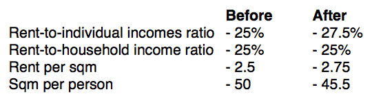
In this scenario what measures can signal a supply-side squeeze? Clearly we need to be looking at an increase in the rent to individual income and a decline in the sqm per person as evidence of a supply side squeeze.
But once you introduce two more critical features to the model – geography and income distribution – things get very interesting.
Geography
We can add geography to our toy model very easily by having the 10 identical homes on a single road heading away from the city centre. They are equally spaced, and the marginal travel cost is $20 per week for each home as distance increases from the city.
In the base case we have 2 people per house willing to spend 34% of their income on a home with zero travel cost (the 1st home on the road).
The first house would rent for $340pw, the next $320, then the third at $300 etc up until the 10th house is rented for $170pw.
Remember, the housing cost (including commuting time) is $340per week for each household. The average and median rent is still $250pw of 25% of household income.
The left graph below summarises this simple linear geographic set up, where a single home is at each point heading away from the city centre, and price a household is willing to pay for each location is falling with distance.
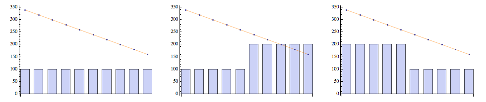
In the situation where all supply is constrained and the population grows by 10%, as in the first example we see that that prices simply increase in accordance with the increased income of the average household.
But what if supply is only constrained over the first half of the road? No new homes can be built in the area occupied by the current 5 closest homes (as stylistically shown in the middle graph above).
The outcome is that the density of the second half of the road increases by 20%.
Prices at each location are identical, but there are now 1.2 homes on average at every position on the road from house 5 onwards.
The mean rent has fallen from $250 to $245 per home because the new homes are only in the inferior locations (the same rent-to-income ratios and same floorspace per capita would exist).
Had there been a ‘greenbelt’ style constraint, in that no new homes could be built in the furthest half of the road (where homes 6 to 10 are located), the number of dwellings in the inner half would have increased by 20% to accommodate the new people. In this case the new average rent would be $255 per dwelling in average. This is because all the new homes are in superior positions. Every single household is still spending 34% of their income, or $340 per week on housing and commuting, and each resident has the same size home.
In either of these cases supply could not be said to be constrained in the city as a whole, despite half of the city being unable to expand dwelling numbers. Yet we see by virtue of location of growth that mean rents will change substantially.
To summarise the impacts of geographically constrained supply we can observe the following metrics
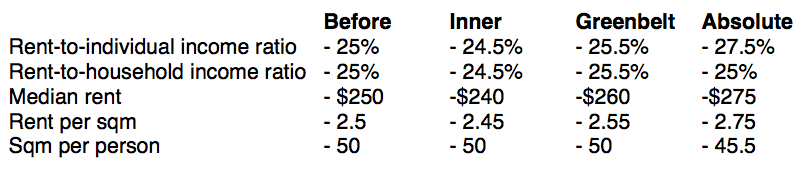
The critical difference between local constraints and absolute city wide constraints is that the sqm of housing per person does not fall. However, this doesn’t mean that some households might be willing to trade household size for location, in which case the housing space per person may shrink in areas close to the city despite the city itself not being supply constrained and the fringes being able to be easily developed.
Income distribution
If we add another dimension to this toy model in the form of a stylised income distribution. Income differences allow wealthier individuals to use their income to outbid for superior locations.
Say the average individual still earns $52,000 per year ($1000pw), but that the wealthiest individual earns $125,000 and the poorest $13,400. Each household in between earns 80% of the previous household, starting at the wealthiest.
We also convert the $20/week incremental commute cost to a commute-time cost based on the wage rate of each household. Thus the commute cost to the first home costs $20 for the average income earner, but $48 of time for the high income earner, and just $5.17 for the lowest income earner.
What happens in this situation is that households sort themselves into inferior/superior locations based on incomes. But it also means that the rental gradient is much steeper than the income gradient.
Let’s see how this works.
Imagine that only the worst located home is vacant, and only the poorest household is in need of a home. How does the bargain over rent occur?
Clearly the poor household has no alternative option but to rent an existing home – they can’t buy a piece of land and built their own. Another land owner could build a home for them and rent it, but they would have legitimate worries about being underbid by the current owner of the vacant home. It is optimal for owners of undeveloped land to wait rather than build in order to maintain the rent price level (see here for more details).
The owner of this last home has all the negotiating power to extract the full willingness to pay from the renter, since at a price affordable to this tenant it is also more attractive to wealthier tenants currently residing in more expensive locations. In this case the willingness to pay from the poorest household is 35% of their income minus commuting costs, or $112 per week.
The same logic applies to any of the homes that are vacant at any point in time. Home owners are able to extract rents because of their monopoly bargaining position. We end up with the following situation when we look at rental prices with the population of households with different incomes under differing conditions of restricted supply.
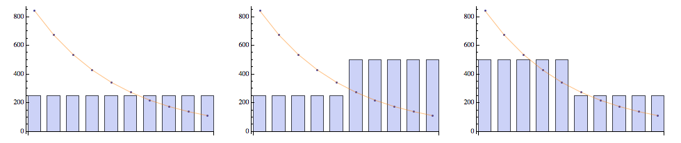
Taking our three types of constraint from the critical indicators in this new case with a 10% population growth and with income inequality are summarised below. Note that while the mean of the income distribution is still $52,000 or $1,000 per week, the presence of very high incomes skews the rent distribution by a large degree. Also not that the income distribution of the additional new population is assumed to be identical to the current population described above.
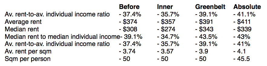
We see that the existence of income inequality actually increases the mean and median measures of rents, despite affordability being identical (34% of income on housing and commuting). The only measure in this case that may indicate a supply constraint is the sqm per person. Any other measure needs to properly control for income and geographical distributions.
All of this begs the next question – why don’t land owners compete rental prices down by building?
Under any of these planning systems there can be vacant developable land at any location in the city. As I’ve discussed elsewhere, the reason is because land development is a one-shot irreversible investment, and as such, the land owner’s optimal choice to to delay investing in housing until such time as it maximises the rate of change in the value of their land. Incentivising construction requires eliminating the value of the option to delay investment. But that is a topic for another post.
Concluding remarks
From this simple model we can see that rents are a function of incomes, willingness to pay for superior locations, commute time and city structure, and ultimately the institutional bargaining power of land owners. Composition of the city matters a great deal, and between-city comparisons of simple metrics in isolation won’t be very informative and may be quite misleading.
Think about it. If all tenants could collectively bargain by agreeing to only pay half the rent they currently pay, and no one would outbid that new halved price in order to move to a better location, then rents would fall. Real wages would rise dramatically, and real land prices would plummet.
If we are seriously about housing affordability, we need to shift the bargaining power towards tenants. We also need to provide incentives to construct housing rather than hold out for increasing future values of development sites.
Tips, suggestions, comments and requests to rumplestatskin@gmail.com, plus follow me on Twitter @rumplestatskin